Do you want to use Excel at work? Then you’re in the right place – these features could save you a lot of time and effort when processing data. Using off-the-shelf functions is always preferable to manual calculation, as they greatly help to process data correctly. And last but not least – your Excel skills will greatly improve once you master these functions. Further information, materials and more Excel tutorials can be found in the Training section.

1. Sum

“Sum” is probably the easiest, but also the most important function in Excel. Thanks to it you can sum certain cells or values.

Example 1.

=Sum(A1:A10) or =Sum(A1,A10)

In this example, the first formula sums cells A1 to A10 inclusive, and the second sums only cells A1 and A10. You can also use specific values in the function instead of references.

2. IF

Another relatively simple but very useful function. The formula checks whether a statement is true or false and returns a value according to the statement.

Example 2.

=IF(A2>100, “yes”, “no”)

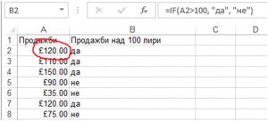
In our example, the formula checks if there are sales over 100 euros in column “A” and if there are returns “yes” against the value in column “B”. If the sale is below 100 euros, the formula returns “no”

3. Sumif

Sumif is a formula with exclusive application. The formula sums values in case they meet a certain condition.

Example 3.

=SUMIF(A1:A20,A2,B1:B20)

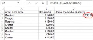
Let us consider the following example. We have sales agents who record a certain number of sales. We want to know the total number of sales for each agent separately. The function =SUMIF(A1:A20,A2,B1:B20) sums the values from cells B1:B20 that correspond to the text in cell A2(in this case “Ivaylo”). I.e. Ivaylo has recorded total sales of £230. In the same way we can use the formula to calculate what turnover the other agents have made.

4. Countif

“Countif” is a very useful function that works in a similar way to “sumif”, i.e. it sums under a certain condition. The difference between sum and count is that the count formula counts the number of cells that have certain information, not the numbers in them.

Example 4.

=COUNTIF(A1:A10,”>100″)

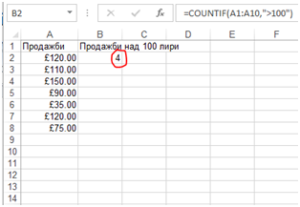
The formula in Example 4 checks how many times sales over 100 pounds were made and returns the number of those sales. You can also include more than one criteria by using countifs for this purpose.

P.S.. If you’re not sure about the syntax of a function, you can always use the Insert function helper (click the function sign next to the formula box, on the left-hand side) In the next example, we’ll demonstrate how it works.

5. Vlookup

Vlookup is an extremely powerful formula that has tremendous application in Excel data processing. A must-have formula for those who need to work with more than one table, to take information from one table and add it to another.

Example 5.

=VLOOKUP(A2,Sheet2!A1:B100,2,0)

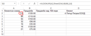
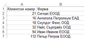
Let’s continue with the same example by adding another column “A”, with customer numbers. Our table has information about our sales and customer numbers, but not the names of our customers. Instead of looking them up one by one from the other Excel table, we can use the formula from Example 4 to look in another table, such as Sheet2, which has info about which company corresponds to which customer number.

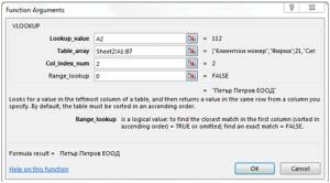
The formula =VLOOKUP(A2,Sheet2!A1:B100,2,0) searches for the value of cell A2 (112 in our example) in the table from Sheet2, columns A1:B100. The function returns the value in the second column. The formula ends with 0 so that Excel can search in a shuffled manner, i.e. not just look at the 2nd row.

We recommend that you construct your own vlookup formula using the insert formula button.

In our case it looks like this:

6. Left, Right, Mid

The left, right, and mid functions have a wide range of uses as they allow you to extract a number of characters from an Excel cell.

Example 6.

=Left(A1,2) or =Mid(A1,4,6) or =Right(A1,5)

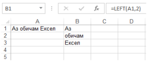
In our example, we use the Left formula to subtract the first 2 characters from left to right. With the right formula we can do the same, but with the characters from right to left. Note that the splice also counts as a character.

7. Trim

Trim is an extremely useful Excel feature because it removes unnecessary splices after words when they are more than 1. It happens very often that the information that is extracted from various databases is full of unnecessary spaces between words. This is a big problem for most Excel formulas because they cannot read the contents in the cell correctly. To get rid of the extra blanks, we use the Trim formula.

Example 7.

=TRIM(A1)

In our example, the =TRIM(A1) formula removes the extra spaces after the words, if any.

8. Concatenate

The concatenate function comes to the rescue when we want to add multiple words or values in a single cell.

Example 8.

=CONCATENATE(B1,” “,B2,” “,B3)

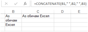
In our example we want to merge the text from cells B1,B2 AND B3. This can be done with the formula =CONCATENATE(B1,B2,B3). This way, however, we won’t have blank spaces after the words. To add blanks between “I” and “love” it is necessary to add the blank space in the formula. This is done by adding quotation marks and spaces in the formula: =CONCATENATE(B1,” “,B2,” “,B3). This way the words will be joined with blank space where needed. Instead of concatenate

P.S.. You can also simply concatenate cells with the & sign:

=B1&” “&B2&” “&B3

Does the same job!

9. LEN

Len is a formula with great application, especially in the construction of more complex formulas.

Example 9.

=Len(C1)

Here we will consider its main function, which is to count the number of characters in a cell. If we take the above example, the function should return you the number 15

10. MAX, MIN

The max and min functions return the largest and smallest number in a table.

Example 10.

=MAX(A2:A8)

=MIN(A2:A8)

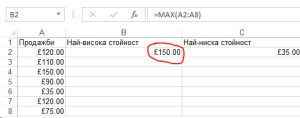
The formula =MAX(A2:A8) returns the largest number from the selected cells in column “A”, and the formula =MIN(A2:A8) gives the smallest.

11. Round

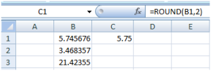
The Round function is very useful when you need to work with round numbers. The Excel can display numbers up to a certain symbol but keeps the original number and uses it in calculations. However, in some cases we need to work with numbers rounded to a certain decimal place. In such cases, the ROUND function comes to the rescue.

Example 11.

=Round(B1,2)

 

© 2024 Atanas Yonkov